
INTRODUCTION
Hospitalisation beds continue to be widely used as a management parameter in hospitals at both the strategic and operational levels, and they are in particularly high demand during pandemic outbreaks because of the need for specialised medical personnel and expensive technical sanitary equipment in intensive care units (ICUs). To offer the greatest patient care and report to public health authorities, an accurate assessment of resources is needed. Preventive measures save lives due to the accuracy of the forecasts. It is well recognised that a hospital is a complex system that is constantly changing within a stochastic environment. The lack of understanding about the propagation of the illness and the effects it has on patients has contributed to an even greater degree of ambiguity than was already there. In this uncertain setting, simulation may be employed alongside other statistical methods to explore complex systems quantitatively. This allows simulation to be a good analytical tool in this uncertain environment. The research published to date has provided a wealth of bibliographical references on the use of simulation models in the process of decision-making in the field of healthcare. Information on the use of simulation models in the medical field is found in some of the recent reviews ( Brailsford et al., 2009; Günal and Pidd, 2010; Katsaliaki and Mustafee, 2011; Mielczarek and Uziałko-Mydlikowska, 2012). The ultimate purpose of these models is to bring the supply of available resources into harmony with the demand for those resources in order to maintain a satisfactory level of human and technological resources while still providing patients with high-quality medical treatment. This method is used to study issues such as patient flow ( Shahani et al., 2008; Kolker, 2009; Zhu et al., 2012; Rodrigues et al., 2018), health service design ( Mallor et al., 2016), and medical staff scheduling ( Erhard et al., 2018). Despite discrepancies between mathematical simulation model assumptions and real health system behaviour reported in the medical literature ( Azcarate et al., 2020), simulation models are useful for analysing complex health system problems.
Typically, the goal of these kinds of simulation models is to replicate the static functioning of the health system, evaluate the patient’s status, and aid in decision-making. The goal is to implement the simulation study’s recommendations into the healthcare system and have them retained in place until either their effectiveness is proven or a better option is found. Simulation models should concentrate on the transition phase and be flexible enough to be combined with dynamic models that learn to manage the illness. Furthermore, the models must pay attention to the transition time in order to get the required knowledge about the patient’s state. This article describes how to build a simulation model that, given enough information about the patient’s current condition, can accurately simulate the patient’s behaviour. In this model, the patient’s progression from one stage to the next (level 1, level 2, and level 3) is simulated using a technique called discrete-event simulation (DES). A patient at level 1 requires urgent medical intervention; a patient at level 2 requires monitoring every 6 hours; and a patient at level 3 is stable with few changes and requires monitoring every 12 hours.
The most popular kind of infectious illness prediction model is a differential equation prediction model ( Grassly and Fraser, 2008; Brauer and Castillo-Chavez, 2012), which is mostly based on population dynamics. The population is broken down into subsets, each of which represents a theoretically feasible state for each given person; each of the three levels: 1, 2, and 3. After estimating the rates at which people move between these states, the population of each state is determined over time. However, these models are complex to grasp and need a huge number of presently unavailable data points for parameter estimation ( Guan et al., 2020). Therefore, if you want an easier way to represent the total number of instances, growth population models are a good choice. Epidemics like A/H1N1 and Ebola have been simulated using these methods (including the logistic, Gompertz, Rosenzweig, and Richards’s models) ( Liu et al., 2015). Customising the simulation model for smart beds is important as it allows for more accurate evaluation and monitoring of patient’s conditions. It enhances the model’s applicability and effectiveness in the specific context of smart bed monitoring. Overall, adapting the simulation model to incorporate smart beds can significantly improve the quality of patient care, enhance healthcare decision-making, and promote more efficient and effective healthcare processes.
THE DES MODEL
Both the utilisation of limited material facilities and resources as well as the facilitation of complicated interactions between various healthcare groups are required for the operation of healthcare systems ( Chahal and Eldabi, 2011; Ben-Tovim et al., 2016; Thorwarth et al., 2016). Healthcare systems are primarily human-based adaptive systems. It is not simple to comprehend, create, or predict complex healthcare systems since they are characterised by a high degree of unpredictability and uncertainty ( Gillespie et al., 2014; Marshall et al., 2015; Arisha and Rashwan, 2016; Lam et al., 2021). This makes it difficult to understand and build these systems.
As healthcare systems continue to advance, there is a growing worry throughout the world about how to improve the quality of treatment while simultaneously lowering costs ( Marshall et al., 2015; Qureshi et al., 2019). Thus, everyday strategic, tactical, and operational decisions review and improve the effectiveness of various healthcare treatments and services ( Chahal and Eldabi, 2011; Marshall et al., 2015). Healthcare professionals need simulation to investigate all conceivable situations ( Chahal et al., 2013; Thorwarth et al., 2016). This will allow them to forecast the influence that these choices will have on the operation of the system.
An imitation of how a system in the actual world functions over the course of time is called a simulation. This may be used to find critical areas and system bottlenecks and answer “what-if” questions regarding real-world scenarios without any practical or cost consequences ( Stahl et al., 2003; Hajjarsaraei et al., 2018; Landa et al., 2018). Simulations may anticipate healthcare treatment outcomes, including behavioural aspects and individualised choices ( Marshall et al., 2015) and the best potential scenario based on output criteria ( Ramwadhdoebe et al., 2009). Using theory or data, a conceptual model represents a system issue ( Abubakar et al., 2020; Davodabadi et al., 2021). Simulation studies start with conceptual models. This conceptual representation needs objectives, inputs, outputs, content, restrictions, assumptions, and simplifications ( Pongjetanapong et al., 2018; Gunal, 2012). Later, the conceptual model is turned into software to help medical professionals comprehend the real-world system’s input and output factors ( Strauss et al., 2021).
The primary contribution of the proposed simulation model is to estimate the health system’s transitional condition by monitoring the elderly or patients’ condition using data provided by smart beds, which, when implemented, will make it possible to anticipate, on a short time scale, decision-making for patients with medical treatment.
Our model includes the following components:
A model of the system and a representation of the patient’s condition in the form of three levels, i.e. level 1, level 2, and level 3.
A prediction of patient state for patients who require any kind of special attention, like home, ward, or ICU.
The ability to reproduce situations using data-driven prediction (based on fitted stochastic models). This research work also describes the use of simulation to aid in a crucial choice that had a direct impact on the well-being of patients. This use of simulation to inform a vital choice was really useful in the real world.
The remaining parts of the article are structured as described below. The DES model is described in the next section, followed by the details of the proposed model. The simulation of the proposed model is described after this section. The outcomes of the simulation model are provided in the section that follows. Finally, the conclusion and future work are presented.
THE PROPOSED MODEL
When experiencing certain symptoms, the typical hospital-goer will either visit the primary care clinic, visit the emergency room, dial an emergency number, or be assessed in a long-term care facility. Depending on their illness, patients are admitted to the ICU or a hospital ward, or hospitalised at home (in medically conditioned beds like smart beds). In each of these three scenarios, the treatment of the patient requires specific allocations of technology. Smart beds and ICU beds are of utmost significance. Figure 1 illustrates the progression behaviour of the proposed model. Patients needing urgent attention are identified as level 1. The severity of the patient’s condition is weak for level 2, and the patient is considered in a normal state for level 3. The proposed model determines whether an individual is in the system to predict if there is any improvement in their health.
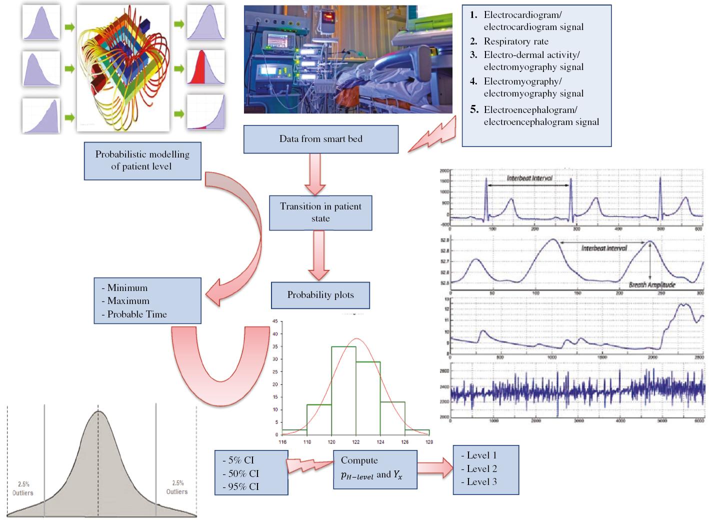
Block diagram of the proposed event driven simulation model for patient level of state monitoring.
Elements of the proposed simulation model
State variables provide a complete description of the simulated system at any given time, while events define the DES model by changing the values of state variables. These two sets work together to produce a full description of the simulated system. The simulation model depicts the progression of patients through different levels. Because of this, there is a requirement for three state variables: patients in each of the three different modalities, i.e. level 1, level 2, and level 3. These are considered input events for the proposed model and are associated with the conclusion of a patient’s state. When an event occurs, the simulation model updates the state variables and performs any necessary calculations to reflect the consequences of the event. The simulation then moves forward in time until the next event occurs, repeating this process until the simulation’s end time is reached. By combining state variables and events, a simulation model can accurately represent the dynamic behaviour of complex systems over time.
Stochastic pattern-based modelling
The time period that patients go through before they need one of the three different levels in healthcare system is depicted in the DES. A common model has been used and fit by assigning the likelihood of the patient state based on the frequencies that have been observed from the smart beds. The cumulative series of the total data [such as heart rate (electrocardiogram/electrocardiogram signal), respiratory rate, skin conductance (electrodermal activity/electromyography signal), muscle current (electromyography/electromyography signal), and brain electrical activity (electroencephalogram/electroencephalogram signal)] from smart bed are used as the data set for fitting an empirical growth model ( Zwietering et al., 1990). This growth model is represented as follows: H(t)=HTexp(−ln(HT/H0)exp(−c(t−t0))). Here, H( t) represents the time dependent parameter of the growth model until time t. H T indicates the patient level at current time. The c value is another parameter that represents the beginning growth rate of the model. The H 0 is the initial level of the state of the patient.
This growth model starts with exponential growth and slows until it reaches a stable state, i.e. level 3. The estimate of the parameters is achieved by reducing the total squared error sum to its smallest value. In actual practise, fitting the data may be accomplished using, for instance, the curve_fit() function found in the optimise module of SciPy in Python or the growth rate package found in R. Both of these packages are available. After the curve H( t) has been fitted, it will be feasible to predict the patient level. Let us assume t i and t i+1 to be two time instances that are consecutive to one another; then, the patient’s level at t i+1 may be estimated as H( t i+1). After that, the simulation model takes a sample from a Poisson form of distribution with a mean of H( t i+1) − H( t i) to predict patient-level transition. However, there may not have been sufficient data available to fit the growth model during the level 3 steady sate of patient. In this scenario, a number of different options are available, each of which is dependent on the application of different models.
The proposed model also changes the growth model to match patient’s smart bed instances. Two things change the projected level. Let us denote f t and f s as state transition and the state severity, respectively. For D( t) the fitted growth curve to the identified level, H( t) becomes equal to f tf sD( t). In light of the fact that there is a lack of data during the steady level 3, this indirect method might also be used and the f s factor would be estimated. The growth model is fitted to data when the number of states changes significantly, indicating exponential development. At this point, both parameters ( f t and f s ) are no longer required since they must both be equal to 1. Estimates of the parameter H T may be derived either directly from the data. Every time a new datum is detected, the curve is adjusted such that it better fits the data.
Probabilistic modelling of patients’ level
Depending on the amount of information at hand, the probabilistic modelling of patients’ level (PMPL) may be simulated using a number of different approaches to estimate probability distributions. All three varieties of simulated levels are simulated here. Triangular distributions are used in the simulation model in the absence or scarcity of data on patients’ PMPL. The lowest, maximum, and most likely times for these distributions are all set according to consensus among experts ( Grassly and Fraser, 2008; Young et al., 2020; Zhou et al., 2020) to provide support for this view. There may be sufficient data to fit probability distributions after one or two transitions. Given that just a tiny fraction of the time when the transition is observed is one of the most notable characteristics of these data, it may lead to the high degree of censorship that they include. This requires re-evaluating the fitting of probability distributions based on the new data. Probability plots simplify the process of selecting the most suitable parametric probability distribution family that accurately represents the data.
After considering all data, including smart bed data, the selected parameters are determined using maximum likelihood. The insights acquired from the operational model indicate that lognormal distribution families provide suitable fits for the data. To be more specific, the PMPL in the hospital may be calculated by applying the technique that has been given, taking into account all three types of patient levels.
In hospitals, the treatment protocols have been modernised to reflect new medical literature, and patient management has improved in hospitals and ICUs. It seems probable that patients as a whole had a beneficial impact as a result of these occurrences. This research has established as a matter of fact that the distributions that were acquired for predicting the patient level are distinct. It has also been observed that the average duration of transitions tends to decline as the patient moves towards level 3. The PMPL of the patients is simulated, which differentiates between the various levels and allows this reality to be reflected in the simulation. The PMPL of the patients is simulated based on the insights acquired from the operational model. Figure 1 shows the block diagram of the proposed event-driven simulation model for patient level of state monitoring.
THE SIMULATION MODEL
Input data
The hospital provides the simulator with an input data file, which the simulator then uses. The data from hospital smart beds are the pieces of information that must be gathered for the health system. These data include heart rate (electrocardiogram/electrocardiogram signal), respiratory rate, skin conductance (electrodermal activity/electromyography signal), muscle current (electromyography/electromyography signal), and brain electrical activity (electroencephalogram/electroencephalogram signal). When a field is blank, it indicates that the related event has not taken place. In other words, if a patient is in level 3 and a transition did not take place, then the level 2 and level 1 fields remain blank. This indicates that the patient did not need special medical care. The information from the smart bed has been recorded in the input data file. As a result, the simulator is able to replicate the patient level in order to initiate the simulation run, which is described in more detail in the next section. It is also possible to conduct the simulation by only being aware of the overall data from smart beds. In this circumstance, the simulator cannot recreate the health system at time 0 of the simulation clock, but it can deduce its state. The accumulated historical series is another kind of input file that the simulator needs, and it may refer to the level of patient state. So the patient pattern may then be calculated with the use of this information, which is used to generate the growth curve that provides the best match.
Probability distribution for level identification
At the time of the most recent change recorded by smart bed data, the simulation clock was initialised to a value of 0. Before that point in time, the simulator will be able to reproduce the past by reading the records included in the record data, but after that point in time, the future will be the one that has to be simulated. It is necessary to initialise it before beginning the simulation since the shift from the past to the future takes place at the very beginning of the process ( Law, 2014). As a result, it is essential to be aware of and simulate the next point in time in the future at which each of these occurrences will take place. As an illustration of the process, let’s take a look at the situation from the hospital smart bed. Let’s say the random variable for PMPL from smart ward is denoted by the letter T. Let’s also say that patient j has been hospitalised in the ward for the past x time units. Consequently, the PMPL for patient j may be characterised by the conditional distribution of variable T provided that T > x such that P{ T > x}= T x whose density function is written as follows: f(x)(1−F(x)) , where f( x) and F( x) are density and distribution functions w.r.t. time t, respectively. When a value t is chosen at random instant from this probability distribution, the level of patient j is calculated as time t − x, and this information is added to the log file. Then, all other levels and transitions are captured in every day may be determined using the fitted growth curve. These transitions may follow a stationary pattern throughout the course of the next 24 h or they may follow a non-stationary trend if, for instance, there is a major drop in the number of transitions during the night.
In the case of level 1, p H−Level represents the approximate probability of level where attention is needed which may be approximated by applying a probability distribution to the random variable Y whose value is generated form smart bed. After x time units, there is a possibility that the patient will have a new transition, and this probability is equal to Y x = P such that Y > x. A patient state x time units ago will be transferred to the ICU with a probability equal to p H−Level,x = p H−Level,x × Y x / T x . It is determined for each smart bed based on a comparison of a uniform random number with the value p H−Level,x . The decision to move the patient state from one level to another is based on the conditional distribution (Y | Y〉x) .
SIMULATION OUTPUT
The simulation model incorporates not one but two distinct forms of randomisation. The number of patients states whose PMPL is calculated. It is possible to acquire the distribution from smart bed data by running the simulation. The confidence bands are presented in visuals once the percentiles of the distribution have been calculated by the simulator. In our experiments the following percentiles are determined: the 5th percentile, the 50th percentile, and the 95th percentile. We have following input to the simulator: heart rate (electrocardiogram/electrocardiogram signal), respiratory rate, skin conductance (electrodermal activity/electromyography signal), muscle current (electromyography/electromyography signal), and brain electrical activity (electroencephalogram/electroencephalogram signal). Fitting the growth model to the starting data may provide two results. The patient may have random level changes if the curve slope is not steep. The tendency may grow the series exponentially. The variation in the density function can provide valuable information for identifying patient level based on the input from smart bed. In Figure 2, as the time progresses the density function level values decline for all three levels. Figure 3 shows the variation in cumulative transition with respect to the density function. The transitions tend to increase w.r.t density function. However, for level 3 the transition saturates around a particular value which means that the function is no more changing. So the patient’s state is steady. Figure 4a– c plots the cumulative confidence bands in terms of the percentiles of the distribution 5, 50, and 95%, respectively. Figure 5a– c shows the plot of distribution [ f( x)] for x values in level 1, level 2, and level 3 scenario, respectively. Tables 1– 3 present the statistical values for 5, 50, and 95% confidence band, respectively. Tables 4– 6 present values of different parameters for 10 records in 5, 50, and 95% confidence band, respectively.


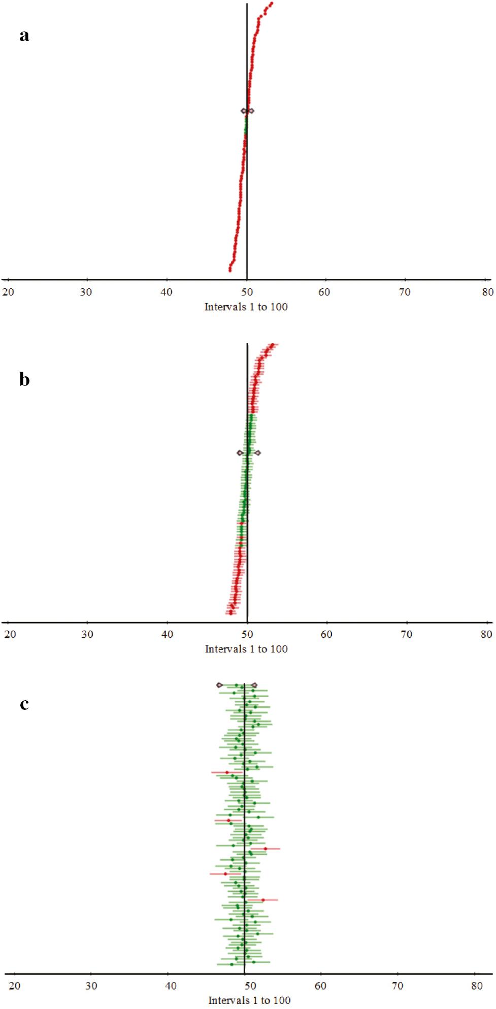
Cumulative confidence bands in terms of the percentiles of the distribution: (a) 5%, (b) 50%, and (c) 95%.
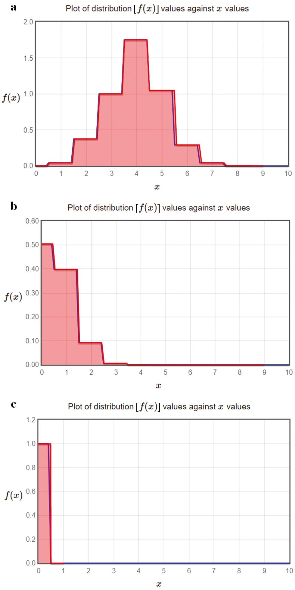
Plot of distribution [ f( x)] against x values in (a) level 1 scenario, (b) level 2 scenario, and (c) level 3 scenario.
Statistical values for 5% confidence band.
| Statistics | Value |
|---|---|
| Sample size | 100 |
| Mean | 50.215 |
| Standard error | 1.073 |
| 5% Lower limit | 50.148 |
| 5% Upper limit | 50.283 |
Statistical values for 50% confidence band.
| Statistics | Value |
|---|---|
| Sample size | 100 |
| Mean | 50.215 |
| Standard error | 1.073 |
| 50% Lower limit | 49.492 |
| 50% Upper limit | 50.939 |
Statistical values for 95% confidence band.
| Statistics | Value |
|---|---|
| Sample size | 100 |
| Mean | 49.074 |
| Standard error | 0.973 |
| 95% Lower limit | 47.144 |
| 95% Upper limit | 51.005 |
Values of different parameters for 10 records in 5% confidence band.
| Cumulative data | Severity factor (%) | p H−level | Y x | Patient level of state |
|---|---|---|---|---|
| 43.7708 | 41.45 | 0.193 | 0.893 | Level 1 |
| 79.37795 | 40.34 | 0.232 | 0.911 | Level 1 |
| 63.89423 | 46.54 | 0.171 | 0.834 | Level 1 |
| 46.29408 | 38.67 | 0.391 | 0.538 | Level 2 |
| 42.85993 | 26.78 | 0.448 | 0.469 | Level 2 |
| 55.51202 | 20.56 | 0.387 | 0.587 | Level 2 |
| 60.4042 | 10.76 | 0.5026 | 0.101 | Level 3 |
| 56.48368 | 8.67 | 0.6064 | 0.192 | Level 3 |
| 72.40579 | 5.78 | 0.5103 | 0.172 | Level 3 |
| 47.42375 | 4.24 | 0.5141 | 0.138 | Level 3 |
Values of different parameters for 10 records in 5% confidence band.
| Cumulative data | Severity factor | p H−level | Y x | Patient level of state |
|---|---|---|---|---|
| 69.5807 | 44.44605 | 0.141 | 0.826 | Level 1 |
| 47.00953 | 43.22984 | 0.14 | 0.914 | Level 1 |
| 41.23474 | 39.06625 | 0.418 | 0.581 | Level 2 |
| 51.59874 | 41.40005 | 0.12 | 0.807 | Level 1 |
| 50.0783 | 28.37238 | 0.316 | 0.501 | Level 2 |
| 74.04077 | 21.55724 | 0.399 | 0.457 | Level 2 |
| 48.93099 | 10.81955 | 0.639 | 0.078 | Level 3 |
| 57.97806 | 8.529569 | 0.779 | 0.169 | Level 3 |
| 55.47518 | 5.363046 | 0.519 | 0.149 | Level 3 |
| 50.2198 | 3.675695 | 0.559 | 0.115 | Level 3 |
Values of different parameters for 10 records in 5% confidence band.
| Data 95% | Severity factor | p H−level | Y x | Patient level of state |
|---|---|---|---|---|
| 60.94817 | 33.5745 | 0.398 | 0.504 | Level 2 |
| 51.30119 | 32.6754 | 0.438 | 0.496 | Level 2 |
| 38.37412 | 49.5974 | 0.278 | 0.926 | Level 1 |
| 46.86485 | 41.3227 | 0.117 | 0.944 | Level 1 |
| 52.17673 | 21.6918 | 0.257 | 0.867 | Level 2 |
| 41.46158 | 16.6536 | 0.596 | 0.081 | Level 3 |
| 45.93639 | 8.7156 | 0.636 | 0.172 | Level 3 |
| 54.36403 | 7.0227 | 0.675 | 0.152 | Level 3 |
| 35.16061 | 4.6818 | 0.714 | 0.118 | Level 3 |
| 60.50745 | 3.4344 | 0.753 | 0.195 | Level 3 |
Observations reveal that when there is an increased frequency of transitions between levels over time, the resulting curve exhibits a non-linear pattern. Due to insufficient data for accurately estimating the PMPL of patients, a triangular distribution is employed as it offers greater accuracy. Additionally, it is observed that the shortest duration, longest duration, and the most probable duration between the two levels are estimated to be 8, 15, and 10 min, respectively. To account for the changing levels in the pattern, a severity factor needs to be incorporated. This factor reflects the varying intensity or severity of the transitions between levels. This factor should be equal to 4, 20, and 40% for level 3, level 2, and level 1, respectively. As was the case with the level 1 situations, the initial fits involve specifying the maximum number of transitions from H t. This is important since the growth model curve climbs exponentially. According to the experimental findings if there were already sufficient data to estimate the PMPL in all levels it is feasible to model the development of the actual progression.
When monitoring patients using a smart bed, it might be helpful to have a DES model on hand as an instrument. The model may be used to simulate a variety of different situations and evaluate the effect that a number of different treatments have on patient outcomes. It is possible, for instance, to use the model to examine the influence of various bed rest postures and turning schedules on the incidence of pressure ulcers, in addition to the incidence of other disorders such as respiratory distress and fluid accumulation.
In addition, the model may be used to investigate staffing requirements and optimise workflow in order to enhance patient care and prevent injuries. A simulation model may help doctors choose the best patient treatment. This entails evaluating staffing levels, scheduling regulations, and protocols to identify the best way for time management, resource allocation, and success.
Using real-world data and patient observations with the simulation model can help improve patient care. The model will accurately replicate real-world scenarios. The model can aid data-driven decision-making. Nevertheless, it is crucial for healthcare professionals to ultimately depend on their own professional expertise and judgement when providing patient care. The incorporation of simulation models within the healthcare industry is widely recognised as a valuable tool for enhancing the effectiveness of decision-making processes. It provides insights into patient severity levels, helps evaluate resource requirements, and aids in optimising medical treatment processes.
CONCLUSION
In the healthcare sector, it is crucial to have accurate projections of the resources required for taking care of patients, which will lessen the amount of strain placed on the system as well as the stress experienced by those working in the industry. In this article, a DES model is presented that was built for monitoring the severity level of patients. The growth model is used to provide predictions, either directly or indirectly, for different levels. These forecasts are used to feed the simulation model. An enhancement to the simulation model can be made so that it can make more accurate predictions. In addition, variables that impact the PMPL are being analysed in order to construct a more complete simulated model that can be customised for the smart bed. The simulation model may be changed to offer an accurate evaluation of smart bed monitoring because of its simple design. The proposed simulation models provide this advantage. The simulation model is data-driven, which means that PMPL may be calculated from the data. The model may also simulate human input, allowing the user to explore different options. Data quality affects projection accuracy. The simulation model emphasises the transition phase instead of the stable state, which is usual in simulation studies, or transition periods following regeneration points. This is a technical and methodological difference. The simulation model is unique. This transition phase that the simulator has simulated is one of the time-series types without any regeneration points, and biological signals are dependent on time. As a result, the precise description of the starting condition of the health system plays a significant role. The simulation of PMPL for smart beds has proven to be an important step in projecting the dynamics of the health system in a smooth manner.